Conditional formatting helps identify an Excel spreadsheet’s data by highlighting cells based on certain criteria provided by the user. This feature overrides any default cell styles in the worksheet when the cell value matches the criteria. This blog will discuss how to implement conditional formatting in Excel spreadsheets using Syncfusion’s .NET Excel Library in C#.
The following types of conditional formatting are available in Excel Library:

Enjoy a smooth experience with Syncfusion’s Excel Library! Get started with a few lines of code and without Microsoft or interop dependencies.
Cell rules
In this type, conditional formatting is applied directly to specific cells based on the cell value. The specified formatting will be applied if the cell value matches the condition. For example, you can use this type of formatting to highlight expenses in an expense report. When an expense falls below $10,000, you can highlight it green, or if it is above that threshold, it can be highlighted red. Doing so provides visual distinctions between low and high expenses.
The following code example shows how to highlight cell values with conditional formatting using specific cell rules.
using System.IO;
using Syncfusion.XlsIO;

namespace Create_Conditional_Format
{
    class Program
    {
        static void Main(string[] args)
        {
            using (ExcelEngine excelEngine = new ExcelEngine())
            {
                IApplication application = excelEngine.Excel;
                application.DefaultVersion = ExcelVersion.Xlsx;
                IWorkbook workbook = application.Workbooks.Create(1);
                IWorksheet worksheet = workbook.Worksheets[0];

                //Applying conditional formatting to "A1".
                IConditionalFormats condition = worksheet.Range["A1"].ConditionalFormats;
                IConditionalFormat condition1 = condition.AddCondition();

                //Represents conditional format rule that the value in the target range should be between 10 and 20.
                condition1.FormatType = ExcelCFType.CellValue;
                condition1.Operator = ExcelComparisonOperator.Between;
                condition1.FirstFormula = "10";
                condition1.SecondFormula = "20";
                worksheet.Range["A1"].Text = "Enter a number between 10 and 20";

                //Setting back color and font style to be applied for the target range.
                condition1.BackColor = ExcelKnownColors.Light_orange;
                condition1.IsBold = true;
                condition1.IsItalic = true;

                //Applying conditional formatting to "A3".
                condition = worksheet.Range["A3"].ConditionalFormats;
                IConditionalFormat condition2 = condition.AddCondition();

                //Represents conditional format rule that the cell value should be 1000.
                condition2.FormatType = ExcelCFType.CellValue;
                condition2.Operator = ExcelComparisonOperator.Equal;
                condition2.FirstFormula = "1000";
                worksheet.Range["A3"].Text = "Enter the Number as 1000";

                //Setting fill pattern and back color to the target range.
                condition2.FillPattern = ExcelPattern.LightUpwardDiagonal;
                condition2.BackColor = ExcelKnownColors.Yellow;

                //Applying conditional formatting to "A5".
                condition = worksheet.Range["A5"].ConditionalFormats;
                IConditionalFormat condition3 = condition.AddCondition();

                //Setting conditional format rule that the cell value for the target range should be less than or equal to 1000.
                condition3.FormatType = ExcelCFType.CellValue;
                condition3.Operator = ExcelComparisonOperator.LessOrEqual;
                condition3.FirstFormula = "1000";
                worksheet.Range["A5"].Text = "Enter a Number which is less than or equal to 1000";

                //Setting back color to target range.
                condition3.BackColor = ExcelKnownColors.Light_green;

                #region Save
                //Saving the workbook.
                FileStream outputStream = new FileStream("ConditionalFormat.xlsx", FileMode.Create, FileAccess.Write);
                workbook.SaveAs(outputStream);
                #endregion

                //Dispose streams.
                outputStream.Dispose();
            }
        }
    }
}
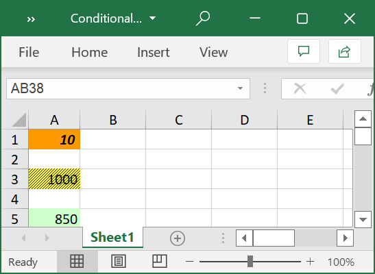
After applying the cell values in the Excel spreadsheet generated from the above code example, the output will look like the following screenshot.

Note: For more details, refer to the cell rules in .NET Excel Library documentation.
Top and bottom values
In this type, Excel Library automatically detects the values in a specific range and highlights the top and bottom n number of cells based on the conditional formatting styles.
You can highlight the top 10 expenses in an expense report using this conditional formatting type. You can also use this formatting to highlight unique and duplicate numbers, as well as numbers above and below an average.
using System.IO;
using Syncfusion.XlsIO;

namespace Top_to_Bottom_Rank
{
    class Program
    {
        static void Main(string[] args)
        {
            using (ExcelEngine excelEngine = new ExcelEngine())
            {
                IApplication application = excelEngine.Excel;
                application.DefaultVersion = ExcelVersion.Xlsx;
                FileStream inputStream = new FileStream("../../../Data/InputTemplate.xlsx", FileMode.Open, FileAccess.Read);
                IWorkbook workbook = application.Workbooks.Open(inputStream);
                IWorksheet worksheet = workbook.Worksheets[0];

                //Applying conditional formatting to "N6:N35".
                IConditionalFormats formats = worksheet.Range["N6:N35"].ConditionalFormats;
                IConditionalFormat format = formats.AddCondition();

                //Applying top or bottom rule in the conditional formatting.
                format.FormatType = ExcelCFType.TopBottom;
                ITopBottom topBottom = format.TopBottom;

                //Set type as Top for TopBottom rule.
                topBottom.Type = ExcelCFTopBottomType.Top;

                //Set rank value for the TopBottom rule.
                topBottom.Rank = 10;

                //Set color for Conditional Formattting.
                format.BackColorRGB = Syncfusion.Drawing.Color.FromArgb(51, 153, 102);

                #region Save
                //Saving the workbook.
                FileStream outputStream = new FileStream("TopToBottomRank.xlsx", FileMode.Create, FileAccess.Write);
                workbook.SaveAs(outputStream);
                #endregion

                //Dispose streams.
                outputStream.Dispose();
                inputStream.Dispose();
            }
        }
    }
}
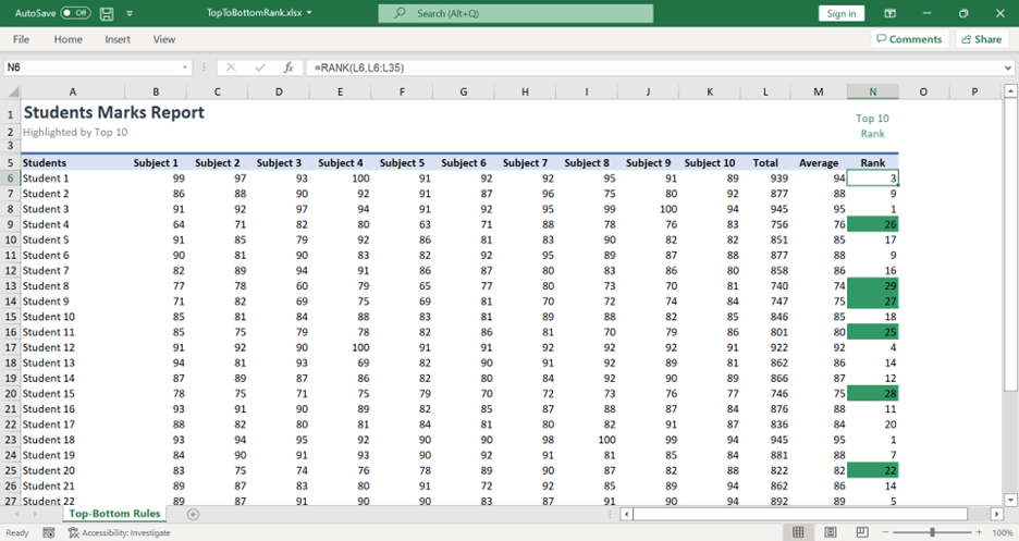
The output of the above code example will look like the following screenshot.

Note: For more details, refer to the top and bottom values formatting in .NET Excel Library documentation.
Color scales
While using color scale formatting, the cell color intensity will increase from bottom to top values in a cell range between specified colors. This helps identify one cell value’s place within a larger set of data. For example, we can highlight a yearly sales report divided by month with a color scale to show which months had higher or lower sales and compare other months’ sales through cell color intensity.
Refer to the following code example.
//Create a color scale for the data in the specified range.
IConditionalFormats conditionalFormats = worksheet.Range["D7:D46"].ConditionalFormats;
IConditionalFormat conditionalFormat = conditionalFormats.AddCondition();
conditionalFormat.FormatType = ExcelCFType.ColorScale;
IColorScale colorScale = conditionalFormat.ColorScale;

//Set a three-color scale and its constraints.
colorScale.SetConditionCount(3);
colorScale.Criteria[0].FormatColorRGB = Color.FromArgb(230, 197, 218);
colorScale.Criteria[0].Type = ConditionValueType.LowestValue;
colorScale.Criteria[0].Value = "0";

colorScale.Criteria[1].FormatColorRGB = Color.FromArgb(244, 210, 178);
colorScale.Criteria[1].Type = ConditionValueType.Percentile;
colorScale.Criteria[1].Value = "50";

colorScale.Criteria[2].FormatColorRGB = Color.FromArgb(245, 247, 171);
colorScale.Criteria[2].Type = ConditionValueType.HighestValue;
colorScale.Criteria[2].Value = "0";
Note: For more details, refer to the color scales in .NET Excel Library documentation.
Data bars
In this type, a color band is used inside a cell to show the top-to-bottom values in a specified cell range. Similar to a color scale, data bars also highlight the data but with a single color, whereas the color scale uses two or three colors. You can say data bars are a minimal version of bar charts in which bars are used inside a cell instead of on a separate chart in the Excel worksheet. An example of when to use data bars would be to highlight and present the value of a stock for over a period of time. The growth or decline of the stock values is easily understood by the different sizes of the data bars.
Refer to the following code example.
//Create data bars for the data in a specified range.
IConditionalFormats conditionalFormats = worksheet.Range["C7:C46"].ConditionalFormats;
IConditionalFormat conditionalFormat = conditionalFormats.AddCondition();
conditionalFormat.FormatType = ExcelCFType.DataBar;
IDataBar dataBar = conditionalFormat.DataBar;

//Set the constraints.
dataBar.MinPoint.Type = ConditionValueType.LowestValue;
dataBar.MaxPoint.Type = ConditionValueType.HighestValue;

//Set color for DataBar.
dataBar.BarColor = Color.FromArgb(156, 208, 243);

//Hide the data bar values.
dataBar.ShowValue = false;
dataBar.BarColor = Color.Aqua;
Note: For more details, refer to data bars in .NET Excel Library documentation.
Icon sets
Icon sets help group large amounts of data with icons, each with a specific threshold value. Similar to cell-rule formatting, when a specified condition matches, an icon is applied to the cell instead of any other formatting. For example, we can highlight an employee rating with five stars when the employee’s performance is extraordinary or noted with two stars when the performance is poor. In such a report, highlighting data with icons will be more suitable than using cell colors.
Refer to the following code example.
//Create icon sets for the data in a specified range.
IConditionalFormats conditionalFormats = worksheet.Range["E7:E46"].ConditionalFormats;
IConditionalFormat conditionalFormat = conditionalFormats.AddCondition();
conditionalFormat.FormatType = ExcelCFType.IconSet;
IIconSet iconSet = conditionalFormat.IconSet;

//Apply three symbol icons and hide the data in the specified range.
iconSet.IconSet = ExcelIconSetType.ThreeSymbols;
iconSet.IconCriteria[1].Type = ConditionValueType.Percent;
iconSet.IconCriteria[1].Value = "50";
iconSet.IconCriteria[2].Type = ConditionValueType.Percent;
iconSet.IconCriteria[2].Value = "50";
iconSet.ShowIconOnly = true;
The following code example shows how to use color scales, data bars, and icon sets to highlight data.
using System.IO;
using Syncfusion.XlsIO;
using Syncfusion.Drawing;

namespace Advanced_Conditional_Formats
{
    class Program
    {
        static void Main(string[] args)
        {
            using (ExcelEngine excelEngine = new ExcelEngine())
            {
                IApplication application = excelEngine.Excel;
                application.DefaultVersion = ExcelVersion.Xlsx;
                FileStream inputStream = new FileStream("../../../Data/InputTemplate.xlsx", FileMode.Open, FileAccess.Read);
                IWorkbook workbook = application.Workbooks.Open(inputStream, ExcelOpenType.Automatic);
                IWorksheet worksheet = workbook.Worksheets[0];

                //Create data bars for the data in the specified range.
                IConditionalFormats conditionalFormats = worksheet.Range["C7:C46"].ConditionalFormats;
                IConditionalFormat conditionalFormat = conditionalFormats.AddCondition();
                conditionalFormat.FormatType = ExcelCFType.DataBar;
                IDataBar dataBar = conditionalFormat.DataBar;

                //Set the constraints.
                dataBar.MinPoint.Type = ConditionValueType.LowestValue;
                dataBar.MaxPoint.Type = ConditionValueType.HighestValue;

                //Set color for bar.
                dataBar.BarColor = Color.FromArgb(156, 208, 243);

                //Hide the values in the data bar.
                dataBar.ShowValue = false;
                dataBar.BarColor = Color.Aqua;

                //Create color scales for the data in a specified range.
                conditionalFormats = worksheet.Range["D7:D46"].ConditionalFormats;
                conditionalFormat = conditionalFormats.AddCondition();
                conditionalFormat.FormatType = ExcelCFType.ColorScale;
                IColorScale colorScale = conditionalFormat.ColorScale;

                //Sets three-color scale.
                colorScale.SetConditionCount(3);
                colorScale.Criteria[0].FormatColorRGB = Color.FromArgb(230, 197, 218);
                colorScale.Criteria[0].Type = ConditionValueType.LowestValue;
                colorScale.Criteria[0].Value = "0";

                colorScale.Criteria[1].FormatColorRGB = Color.FromArgb(244, 210, 178);
                colorScale.Criteria[1].Type = ConditionValueType.Percentile;
                colorScale.Criteria[1].Value = "50";

                colorScale.Criteria[2].FormatColorRGB = Color.FromArgb(245, 247, 171);
                colorScale.Criteria[2].Type = ConditionValueType.HighestValue;
                colorScale.Criteria[2].Value = "0";

                conditionalFormat.FirstFormulaR1C1 = "=R[1]C[0]";
                conditionalFormat.SecondFormulaR1C1 = "=R[1]C[1]";

                //Create icon sets for the data in the specified range.
                conditionalFormats = worksheet.Range["E7:E46"].ConditionalFormats;
                conditionalFormat = conditionalFormats.AddCondition();
                conditionalFormat.FormatType = ExcelCFType.IconSet;
                IIconSet iconSet = conditionalFormat.IconSet;

                //Apply three symbol icons and hide the data in the specified range.
                iconSet.IconSet = ExcelIconSetType.ThreeSymbols;
                iconSet.IconCriteria[1].Type = ConditionValueType.Percent;
                iconSet.IconCriteria[1].Value = "50";
                iconSet.IconCriteria[2].Type = ConditionValueType.Percent;
                iconSet.IconCriteria[2].Value = "50";
                iconSet.ShowIconOnly = true;

                #region Save
                //Save the workbook.
                FileStream outputStream = new FileStream("AdvancedCF.xlsx", FileMode.Create, FileAccess.Write);
                workbook.SaveAs(outputStream);
                #endregion

                //Dispose streams.
                outputStream.Dispose();
                inputStream.Dispose();
            }
        }
    }
}
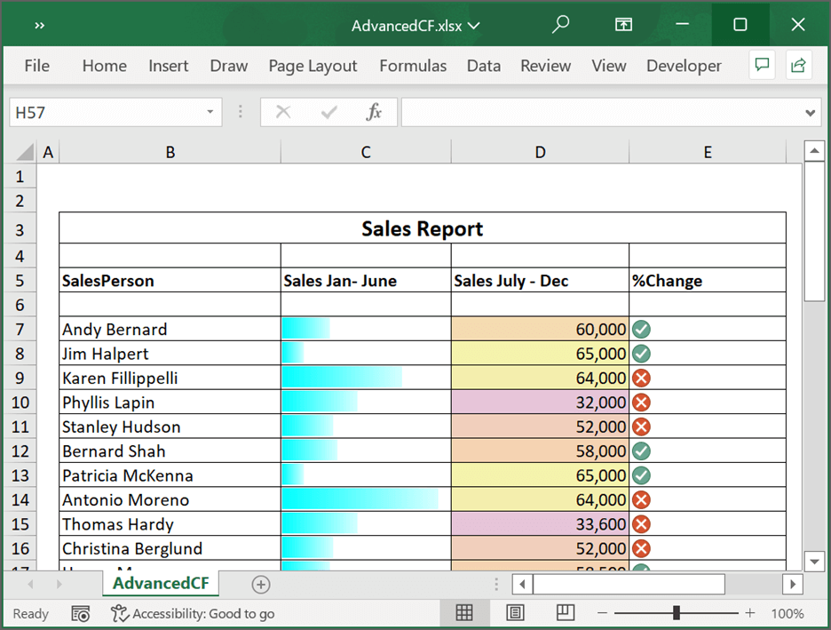
The output of the above code example looks like the following screenshot.

Note: For more details, refer to the icon sets in .NET Excel Library documentation.
GitHub samples
You can download examples of highlighting data with conditional formatting in C# from this GitHub repository.

Don't settle for ordinary spreadsheet solutions. Switch to Syncfusion and upgrade the way you handle Excel files in your apps!
Conclusion
Syncfusion Excel (XlsIO) Library provides support to highlight Excel data using C#. Take a moment to peruse the documentation where you’ll find other formatting options and features like importing and exporting data, data validation, tables, and charts with accompanying code samples.
Using the Excel Library, you can export Excel data to PDF, image, data table, CSV, TSV, HTML, collections of objects, ODS, JSON, and more file formats.
If you are new to our Excel Library, we highly recommend you follow our getting started guide.
Are you already a Syncfusion user? You can download the product setup here. If you’re not yet a Syncfusion user, you can download a free, 30-day trial here.
Please let us know your thoughts in the comments section below. If you have questions about these features, contact us through our support forum, support portal, or feedback portal. We are always happy to assist you!
Related blogs
- 6 Easy Ways to Export Data to Excel in C#
- How to Export Data from SQL Server to Excel Table in C#
- Export Data from Collection to Excel and Group It in C#
- Export Data to a Predefined Excel Template in C#
